tip <-read.csv("../../data/tip.csv")
print(head(tip))

      Name Gender Food.preferance Tip
1    Aanya Female             Veg   0
2     Adit   Male             Veg   0
3    Aditi Female             Veg  20
4    Akash   Male         Non-veg   0
5  Akshita Female         Non-veg   0
6 Anandita Female         Non-veg   0

Research Question: Is there a significant difference in the average tip amount given by non-vegetarians compared to vegetarians?

inspect(tip)


categorical variables:  
             name     class levels  n missing
1            Name character     58 60       0
2          Gender character      2 60       0
3 Food.preferance character      2 60       0
                                   distribution
1 Ananya (3.3%), Simran (3.3%) ...             
2 Female (50%), Male (50%)                     
3 Non-veg (50%), Veg (50%)                     

quantitative variables:  
  name   class min Q1 median Q3 max     mean       sd  n missing
1  Tip integer   0  0      0 20 100 11.16667 17.83556 60       0

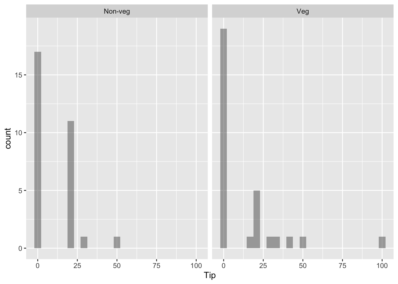
tip %>% crosstable(Tip~Food.preferance) %>% as_flextable()

label	variable	Food.preferance
label	variable	Non-veg	Veg
Tip	Min / Max	0 / 50.0	0 / 100.0
	Med [IQR]	0 [0;20.0]	0 [0;20.0]
	Mean (std)	10.0 (12.9)	12.3 (21.9)
	N (NA)	30 (0)	30 (0)

mosaic::t_test(Tip~Food.preferance, data=tip)  %>% broom::tidy()

# A tibble: 1 × 10
  estimate estimate1 estimate2 statistic p.value parameter conf.low conf.high
     <dbl>     <dbl>     <dbl>     <dbl>   <dbl>     <dbl>    <dbl>     <dbl>
1    -2.33        10      12.3    -0.503   0.617      46.9    -11.7      6.99
# ℹ 2 more variables: method <chr>, alternative <chr>

mosaic::t_test(Tip~Gender, data=tip)  %>% broom::tidy()

# A tibble: 1 × 10
  estimate estimate1 estimate2 statistic p.value parameter conf.low conf.high
     <dbl>     <dbl>     <dbl>     <dbl>   <dbl>     <dbl>    <dbl>     <dbl>
1        2      12.2      10.2     0.431   0.668      55.8    -7.29      11.3
# ℹ 2 more variables: method <chr>, alternative <chr>

library(dplyr)


tip_modified <- tip %>%
  mutate(Food.preferance = as.factor(Food.preferance))

Qual variables- Gender, Food_Preferance (food_preference*)

Quant variable(s)- Tip

tip_modified %>% gf_histogram(~Tip|Food.preferance)

tip_modified %>%
  gf_density(
    ~ Tip,
    fill = ~ Food.preferance,
    alpha = 0.5,
   
  )

Observations

Most of tips are clustered around the lower end ; Right skew in both cases.

Tips above 50 are rare. One notable outlier in the vegetarian group.
Vegetarians have a broader distribution

Non-vegetarian tips are clustered around 10-25 range, they seem to tip more in this range.

Hypotheses:

H0: μ non-veg=μ veg
Ha: μ non-veg ≠ μ veg

- Check for Normality

tip_modified %>%
  gf_density( ~ Tip,
              fill = ~ Food.preferance,
              alpha = 0.5,
              title = "Tips given by non-vegetarians and vegetarians") %>%
  gf_facet_grid(~ Food.preferance) %>% 
  gf_fitdistr(dist = "dnorm")

Non-vegetarians- Right skewed distribution Vegetarians - Also right skewed but less skewed when compared with non-vegetarians

shapiro.test(tip_modified$Tip[tip_modified$Food.preferance == "Non-veg"])


    Shapiro-Wilk normality test

data:  tip_modified$Tip[tip_modified$Food.preferance == "Non-veg"]
W = 0.71661, p-value = 2.747e-06

p value= 0.000002747

shapiro.test(tip_modified$Tip[tip_modified$Food.preferance == "Veg"])


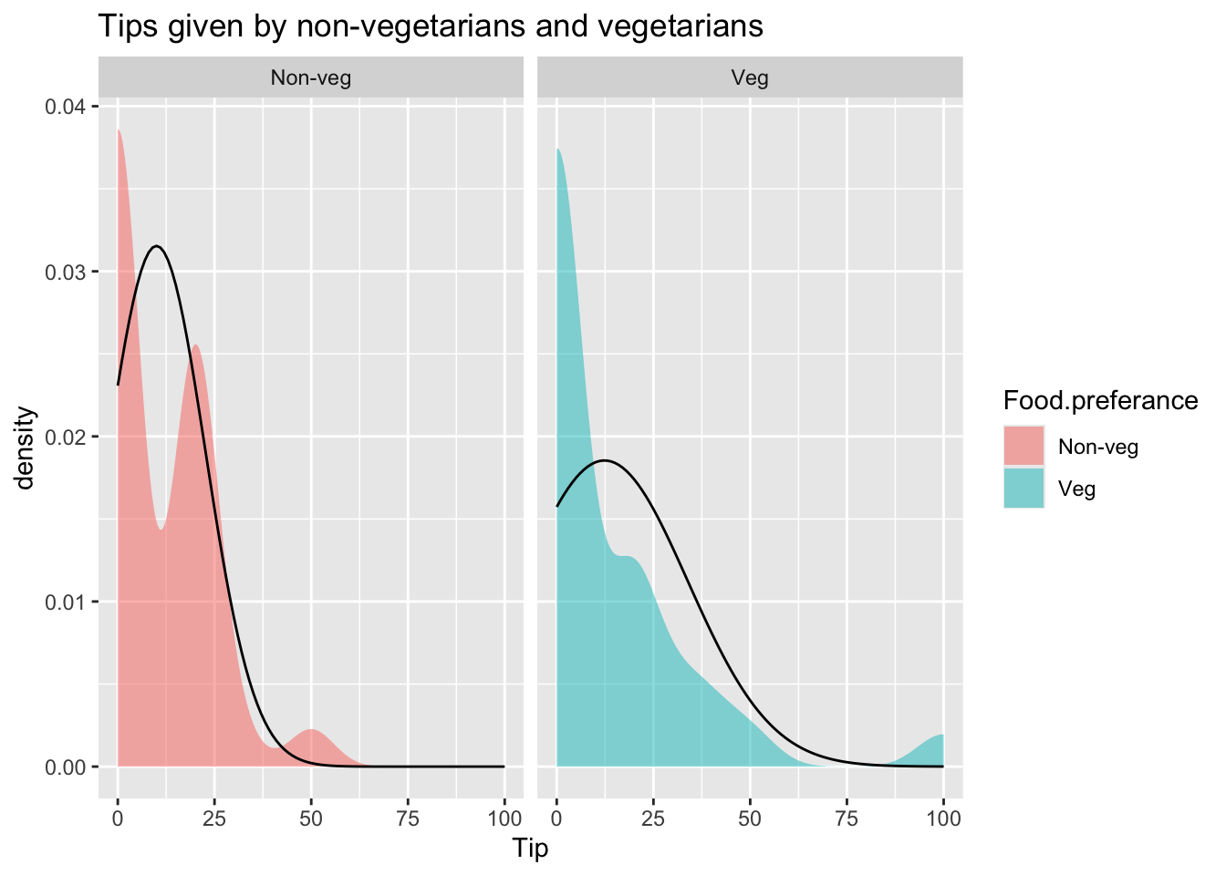
    Shapiro-Wilk normality test

data:  tip_modified$Tip[tip_modified$Food.preferance == "Veg"]
W = 0.6286, p-value = 1.661e-07

p value = 0.0000001661

p-value for both the groups (veg and non-veg) is less than 0.05, as a result we reject the null hypothesis, the data for both groups is not normally distributed.

- Check for Variances

var.test(Tip ~ Food.preferance, data = tip_modified, 
         conf.int = TRUE, conf.level = 0.95) %>% 
  broom::tidy()

Multiple parameters; naming those columns num.df, den.df

# A tibble: 1 × 9
  estimate num.df den.df statistic p.value conf.low conf.high method alternative
     <dbl>  <int>  <int>     <dbl>   <dbl>    <dbl>     <dbl> <chr>  <chr>      
1    0.346     29     29     0.346 0.00554    0.165     0.726 F tes… two.sided

0.00554363 < 0.05, we reject the null hypothesis

-

Difference in Means:

obs_diff_tips <- diffmean(Tip ~ Food.preferance, data = tip_modified) 
obs_diff_tips

diffmean 
2.333333

-Using Parametric t.test

(*data is not Gaussian, variances are different)

–a non-parametric test would be more suitable

–let’s check what we get regardless

mosaic::t_test(Tip ~Food.preferance, data = tip_modified) %>% 
  broom::tidy()

# A tibble: 1 × 10
  estimate estimate1 estimate2 statistic p.value parameter conf.low conf.high
     <dbl>     <dbl>     <dbl>     <dbl>   <dbl>     <dbl>    <dbl>     <dbl>
1    -2.33        10      12.3    -0.503   0.617      46.9    -11.7      6.99
# ℹ 2 more variables: method <chr>, alternative <chr>

p value: 0.6

we fail to reject the null hypothesis, no significant statistical difference between the means of non-vegetarian and vegetarian groups when it comes to tipping.

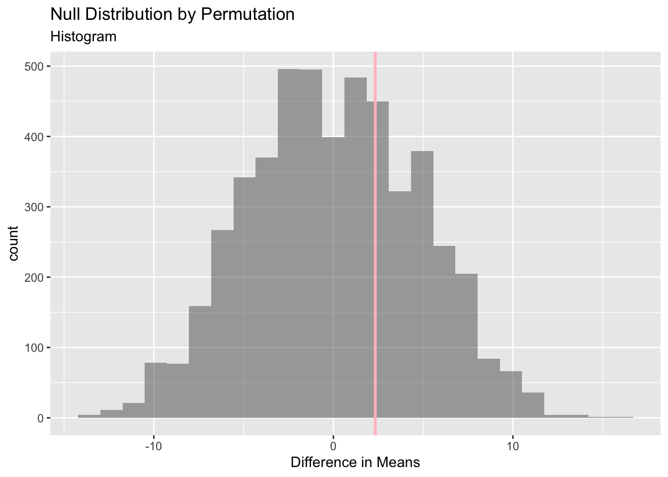
-Permutation test

null_dist_Tip <- 
  do(4999) * diffmean(data =tip_modified, Tip ~ shuffle(Food.preferance))
head(null_dist_Tip, n = 15)

     diffmean
1   5.0000000
2  -8.3333333
3  -1.0000000
4  -8.3333333
5  -4.0000000
6  -0.3333333
7   4.6666667
8  -6.0000000
9   6.3333333
10 -3.0000000
11  5.0000000
12  7.3333333
13 -3.6666667
14 -4.0000000
15  4.6666667

gf_histogram(data = null_dist_Tip, ~ diffmean, bins = 25) %>%
  gf_vline(xintercept = obs_diff_tips, 
           colour = "pink", linewidth = 1,
           title = "Null Distribution by Permutation", 
           subtitle = "Histogram") %>% 
  gf_labs(x = "Difference in Means")

###
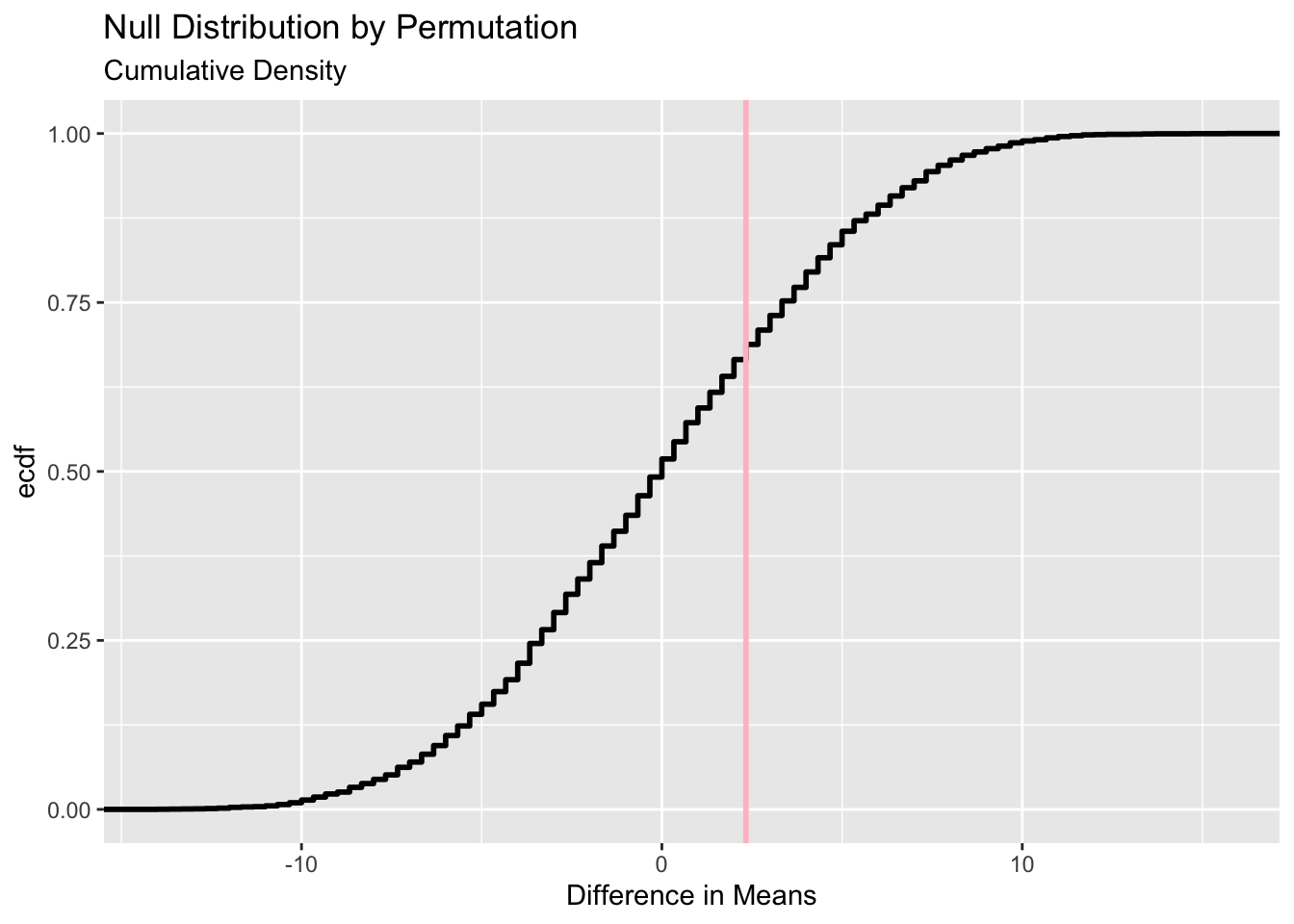
gf_ecdf(data = null_dist_Tip, ~ diffmean, 
        linewidth = 1) %>%
  gf_vline(xintercept = obs_diff_tips, 
           colour = "pink", linewidth = 1,
           title = "Null Distribution by Permutation", 
           subtitle = "Cumulative Density") %>% 
  gf_labs(x = "Difference in Means")

1-prop1(~ diffmean <= obs_diff_tips, data = null_dist_Tip)

prop_TRUE 
    0.312

The observed difference in tips is not beyond anythimg that we could generate with permutations; therefore, there is again no significant different in tips between the vegetarian and non vegetarian groups. We fail to reject the null hypothesis.

————————–

-Mann-Whitney Test

—data is not normally distributed (not Gaussian), and the variances of the two groups are significantly different. This indicates that the assumption of normality is not satisfied, while the assumption of equal variances is satisfied.

– we can do Wilcox.test (test of mean ranks)

wilcox.test(Tip ~ Food.preferance, data = tip_modified, 
            conf.int = TRUE, 
            conf.level = 0.95) %>% 
  broom::tidy()

Warning in wilcox.test.default(x = DATA[[1L]], y = DATA[[2L]], ...): cannot
compute exact p-value with ties

Warning in wilcox.test.default(x = DATA[[1L]], y = DATA[[2L]], ...): cannot
compute exact confidence intervals with ties

# A tibble: 1 × 7
   estimate statistic p.value   conf.low   conf.high method          alternative
      <dbl>     <dbl>   <dbl>      <dbl>       <dbl> <chr>           <chr>      
1 0.0000372       463   0.833 -0.0000335 0.000000989 Wilcoxon rank … two.sided

A-3 tips

Research Question: Is there a significant difference in the average tip amount given by non-vegetarians compared to vegetarians?

Qual variables- Gender, Food_Preferance (food_preference*)

Quant variable(s)- Tip

Observations

Hypotheses:

- Check for Normality

p-value for both the groups (veg and non-veg) is less than 0.05, as a result we reject the null hypothesis, the data for both groups is not normally distributed.

- Check for Variances

0.00554363 < 0.05, we reject the null hypothesis

-

Difference in Means:

-Using Parametric t.test

(*data is not Gaussian, variances are different)

p value: 0.6

we fail to reject the null hypothesis, no significant statistical difference between the means of non-vegetarian and vegetarian groups when it comes to tipping.

-Permutation test

The observed difference in tips is not beyond anythimg that we could generate with permutations; therefore, there is again no significant different in tips between the vegetarian and non vegetarian groups. We fail to reject the null hypothesis.

————————–

-Mann-Whitney Test

p value= 0.8, we fail to reject our null hypothesis again.

hence, there truly is no significant statistical difference between the means of non-veg and veg groups; tips given by both are similar enough.

Research Question: Is there a significant difference in the average tip amount given by non-vegetarians compared to vegetarians?

Qual variables- Gender, Food_Preferance (food_preference*)

Quant variable(s)- Tip

Observations

Hypotheses:

- Check for Normality

p-value for both the groups (veg and non-veg) is less than 0.05, as a result we reject the null hypothesis, the data for both groups is not normally distributed.

- Check for Variances

0.00554363 < 0.05, we reject the null hypothesis

-

Difference in Means:

Inferences

-Using Parametric t.test

(*data is not Gaussian, variances are different)

p value: 0.6

we fail to reject the null hypothesis, no significant statistical difference between the means of non-vegetarian and vegetarian groups when it comes to tipping.

-Permutation test

The observed difference in tips is not beyond anythimg that we could generate with permutations; therefore, there is again no significant different in tips between the vegetarian and non vegetarian groups. We fail to reject the null hypothesis.

————————–

-Mann-Whitney Test

p value= 0.8, we fail to reject our null hypothesis again.

hence, there truly is no significant statistical difference between the means of non-veg and veg groups; tips given by both are similar enough.