Pocket_money <-read.csv("../../data/Pocket_money.csv")
print(head(Pocket_money))

  Sr.no    Name Gender Money_spent  X
1     1   Aagam   Male         150 NA
2     2  Aakash   Male         240 NA
3     3 Aarushi Female         382 NA
4     4 Abheeta Female          60 NA
5     5 Adithya   Male          68 NA
6     6  Aditya   Male         300 NA

Research Question: Is there a significant difference in the average daily pocket money spent by boys and girls?

inspect(Pocket_money)


categorical variables:  
    name     class levels  n missing
1   Name character     82 82       0
2 Gender character      2 82       0
3      X   logical      0  0      82
                                   distribution
1 Aagam (1.2%), Aakash (1.2%) ...              
2 Female (50%), Male (50%)                     
3  (%)                                         

quantitative variables:  
         name   class min     Q1 median     Q3   max     mean         sd  n
1       Sr.no integer   1  21.25   41.5  61.75    82  41.5000   23.81526 82
2 Money_spent integer   0 100.00  264.5 596.25 13000 720.9634 1835.72169 82
  missing
1       0
2       0

Pocket_money %>% crosstable(Money_spent~Gender) %>% as_flextable()

label	variable	Gender
label	variable	Female	Male
Money_spent	Min / Max	0 / 1.3e+04	0 / 1.0e+04
	Med [IQR]	280.0 [85.0;500.0]	250.0 [150.0;842.0]
	Mean (std)	693.3 (2035.8)	748.6 (1636.5)
	N (NA)	41 (0)	41 (0)

mosaic::t_test(Money_spent~Gender, data=Pocket_money)  %>% broom::tidy()

# A tibble: 1 × 10
  estimate estimate1 estimate2 statistic p.value parameter conf.low conf.high
     <dbl>     <dbl>     <dbl>     <dbl>   <dbl>     <dbl>    <dbl>     <dbl>
1    -55.3      693.      749.    -0.136   0.893      76.5    -868.      757.
# ℹ 2 more variables: method <chr>, alternative <chr>

library(dplyr)


pm_modified <- Pocket_money %>%
  mutate(Gender = as.factor(Gender))

Qual variables- Gender

Quant variable(s)- Money_spent

pm_modified %>%
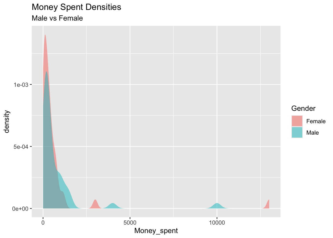
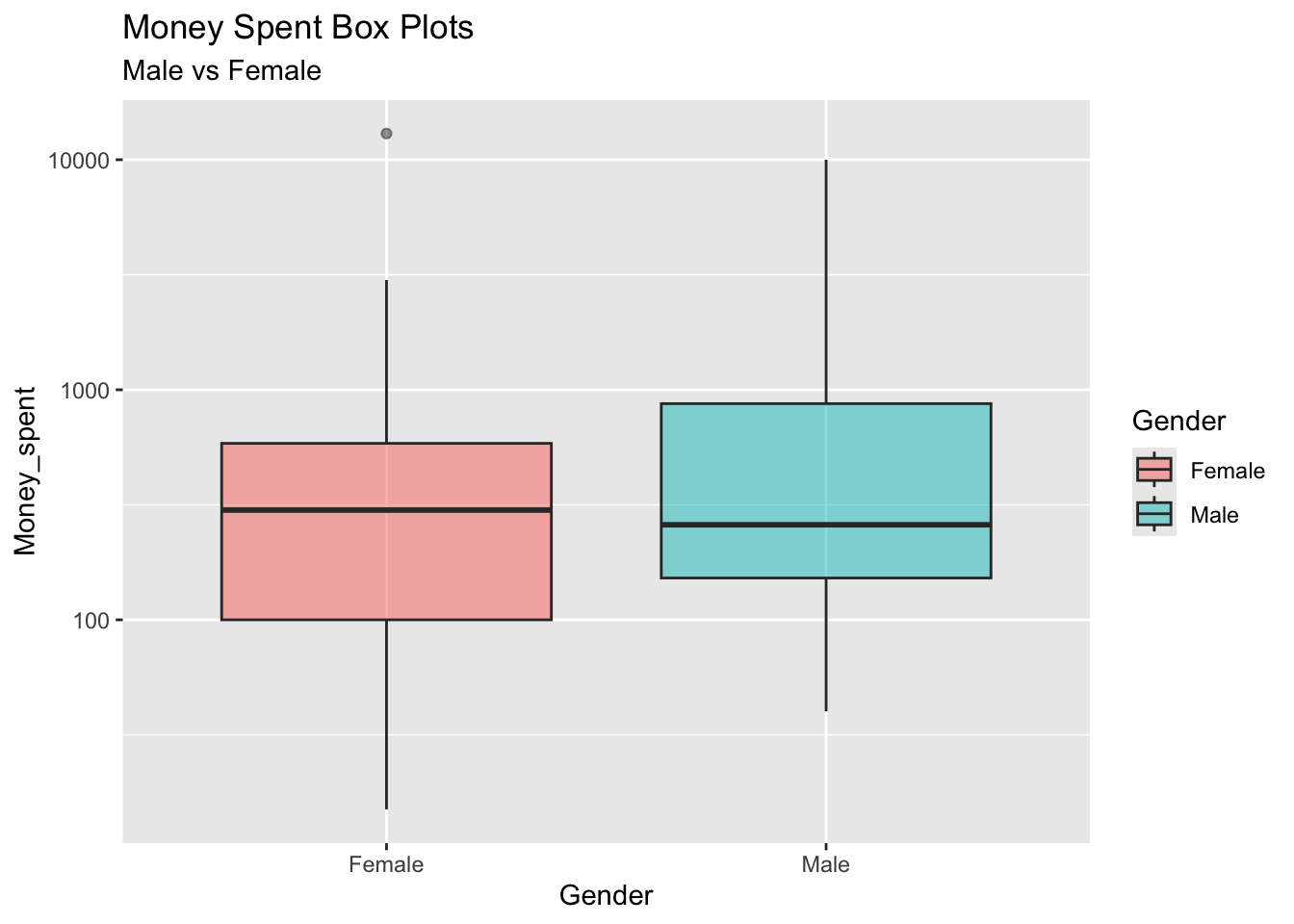
  gf_density(
    ~ Money_spent,
    fill = ~ Gender,
    alpha = 0.5,
    title = "Money Spent Densities",
    subtitle = "Male vs Female"
  )

##
pm_modified %>%
  gf_boxplot(
    Money_spent ~ Gender,
    fill = ~ Gender,
    alpha = 0.5,
    title = "Money Spent Box Plots",
    subtitle = "Male vs Female"
  ) %>% gf_refine(scale_y_log10())

Warning in scale_y_log10(): log-10 transformation introduced infinite values.

Warning: Removed 6 rows containing non-finite outside the scale range
(`stat_boxplot()`).

##
pm_modified %>% count(Gender)

  Gender  n
1 Female 41
2   Male 41

pm_modified %>% 
  group_by(Gender) %>% 
  summarise(mean = mean(Money_spent))

# A tibble: 2 × 2
  Gender  mean
  <fct>  <dbl>
1 Female  693.
2 Male    749.

Observations

Outliers in both groups
Based on median, females spend more money than males.
In the density plot we can see that the distributions overlap to quite an extent, females spend more and there is more variability in male spending.

Hypotheses:

H0: μ male spending=μ female spending
Ha: μ male spending ≠ μ female spending

- Check for Normality

pm_modified %>%
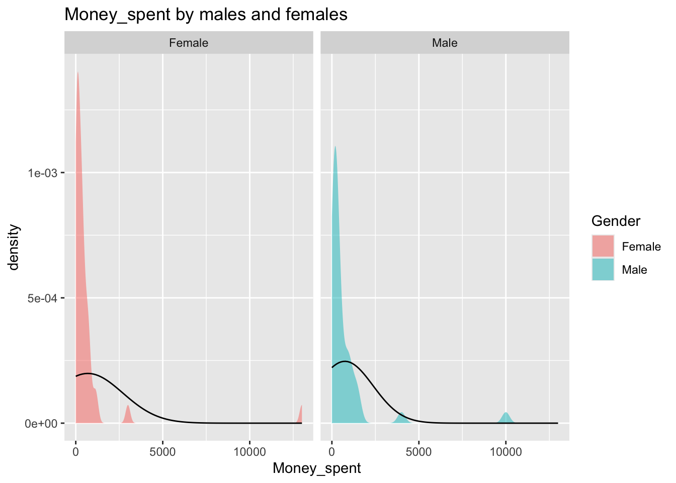
  gf_density( ~ Money_spent,
              fill = ~ Gender,
              alpha = 0.5,
              title = "Money_spent by males and females") %>%
  gf_facet_grid(~ Gender) %>% 
  gf_fitdistr(dist = "dnorm")

both are right skewed and have sharp peaks…

shapiro.test(pm_modified$Money_spent[pm_modified$Gender== "Female"])


    Shapiro-Wilk normality test

data:  pm_modified$Money_spent[pm_modified$Gender == "Female"]
W = 0.29606, p-value = 8.961e-13

p value-> 0.0000000000008961

shapiro.test(pm_modified$Money_spent[pm_modified$Gender== "Male"])


    Shapiro-Wilk normality test

data:  pm_modified$Money_spent[pm_modified$Gender == "Male"]
W = 0.40726, p-value = 1.136e-11

p value-> 0.00000000001136

we can reject the null hypothesis and go forward with our alternative hypothesis based on w values, we can say data is not normally distributed

- Check for Variances

var.test(Money_spent ~ Gender, data = pm_modified, 
         conf.int = TRUE, conf.level = 0.95) %>% 
  broom::tidy()

Multiple parameters; naming those columns num.df, den.df

# A tibble: 1 × 9
  estimate num.df den.df statistic p.value conf.low conf.high method alternative
     <dbl>  <int>  <int>     <dbl>   <dbl>    <dbl>     <dbl> <chr>  <chr>      
1     1.55     40     40      1.55   0.172    0.825      2.90 F tes… two.sided

p value= 0.17 hence variances can be considered approximately equal. we do not reject the null hypothesis.

-

Difference in Means:

obs_diff_pm <- diffmean(Money_spent ~ Gender, data = pm_modified) 
obs_diff_pm

diffmean 
55.29268

-Using Parametric t.test

mosaic::t_test(Money_spent ~Gender, data = pm_modified) %>% 
  broom::tidy()

# A tibble: 1 × 10
  estimate estimate1 estimate2 statistic p.value parameter conf.low conf.high
     <dbl>     <dbl>     <dbl>     <dbl>   <dbl>     <dbl>    <dbl>     <dbl>
1    -55.3      693.      749.    -0.136   0.893      76.5    -868.      757.
# ℹ 2 more variables: method <chr>, alternative <chr>

with a high p value of 0.8, we can say that means of male and female pocket money spendings are not significantly different from one another.

-Using Mann-Whitney

–data variables not distributed normally

wilcox.test(Money_spent ~ Gender, data = pm_modified, 
            conf.int = TRUE, 
            conf.level = 0.95) %>% 
  broom::tidy()

Warning in wilcox.test.default(x = DATA[[1L]], y = DATA[[2L]], ...): cannot
compute exact p-value with ties

Warning in wilcox.test.default(x = DATA[[1L]], y = DATA[[2L]], ...): cannot
compute exact confidence intervals with ties

# A tibble: 1 × 7
  estimate statistic p.value conf.low conf.high method               alternative
     <dbl>     <dbl>   <dbl>    <dbl>     <dbl> <chr>                <chr>      
1    -55.0      746.   0.381    -180.      70.0 Wilcoxon rank sum t… two.sided

p value of 0.3, we fail to reject our null hypothesis.

-Permutation

null_dist_pm <- 
  do(4999) * diffmean(data =pm_modified, Money_spent ~ shuffle(Gender))
head(null_dist_pm, n = 15)

     diffmean
1  -118.56098
2  -695.34146
3    81.68293
4  -435.53659
5   190.36585
6   371.19512
7  -679.73171
8  -555.82927
9   504.17073
10  499.68293
11 -636.80488
12   39.39024
13 -529.39024
14 -517.04878
15 -603.19512

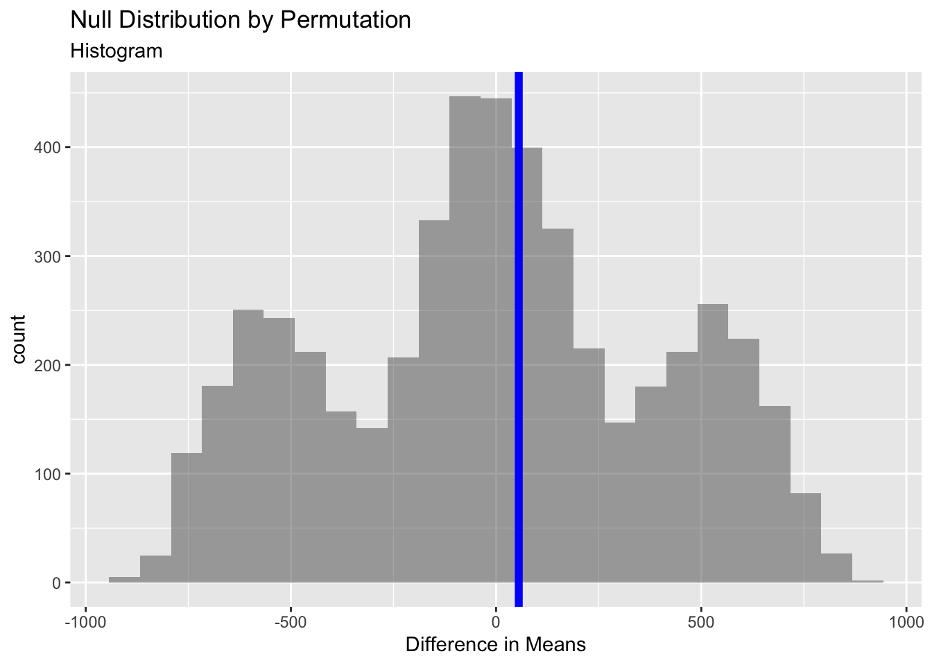
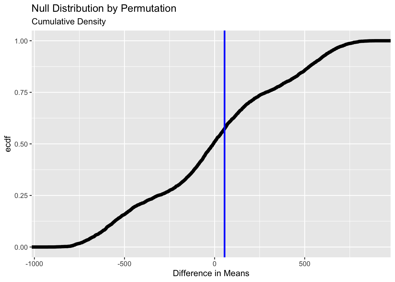
gf_histogram(data = null_dist_pm, ~ diffmean, bins = 25) %>%
  gf_vline(xintercept = obs_diff_pm, 
           colour = "blue", linewidth = 2,
           title = "Null Distribution by Permutation", 
           subtitle = "Histogram") %>% 
  gf_labs(x = "Difference in Means")

###
gf_ecdf(data = null_dist_pm, ~ diffmean, 
        linewidth = 2) %>%
  gf_vline(xintercept = obs_diff_pm, 
           colour = "blue", linewidth = 1,
           title = "Null Distribution by Permutation", 
           subtitle = "Cumulative Density") %>% 
  gf_labs(x = "Difference in Means")

1-prop1(~ diffmean <= obs_diff_pm, data = null_dist_pm)

prop_TRUE 
   0.4262

pocketmoney

Research Question: Is there a significant difference in the average daily pocket money spent by boys and girls?

Qual variables- Gender

Quant variable(s)- Money_spent

Observations

Hypotheses:

- Check for Normality

we can reject the null hypothesis and go forward with our alternative hypothesis based on w values, we can say data is not normally distributed

- Check for Variances

p value= 0.17 hence variances can be considered approximately equal. we do not reject the null hypothesis.

-

Difference in Means:

-Using Parametric t.test

with a high p value of 0.8, we can say that means of male and female pocket money spendings are not significantly different from one another.

-Using Mann-Whitney

p value of 0.3, we fail to reject our null hypothesis.

-Permutation

no strong difference between the groups being compared, female and male pocket money spemdings are approx same.

Research Question: Is there a significant difference in the average daily pocket money spent by boys and girls?

Qual variables- Gender

Quant variable(s)- Money_spent

Observations

Hypotheses:

- Check for Normality

we can reject the null hypothesis and go forward with our alternative hypothesis based on w values, we can say data is not normally distributed

- Check for Variances

p value= 0.17 hence variances can be considered approximately equal. we do not reject the null hypothesis.

-

Difference in Means:

Inferences

-Using Parametric t.test

with a high p value of 0.8, we can say that means of male and female pocket money spendings are not significantly different from one another.

-Using Mann-Whitney

p value of 0.3, we fail to reject our null hypothesis.

-Permutation

no strong difference between the groups being compared, female and male pocket money spemdings are approx same.