cartoons <-read.csv("../../data/cartoonsvs.csv")
print(head(cartoons))
  Participant.ID Gender     Cartoon Rating
1             P1   Male Chota Bheem    8.5
2             P2   Male Chota Bheem    6.0
3             P3   Male Chota Bheem    8.0
4             P4   Male Chota Bheem    7.0
5             P5   Male Chota Bheem    8.0
6             P6   Male Chota Bheem   10.0
## Research Question: Which is better among Doraemon, Dragon Tales, and Chhota Bheem?
library(dplyr)


cartoons_modified <- cartoons %>%
  mutate(Gender = as.factor(Gender)) %>%
  mutate(Cartoon = as.factor(Cartoon))
colnames(cartoons_modified)
[1] "Participant.ID" "Gender" "Cartoon" "Rating"
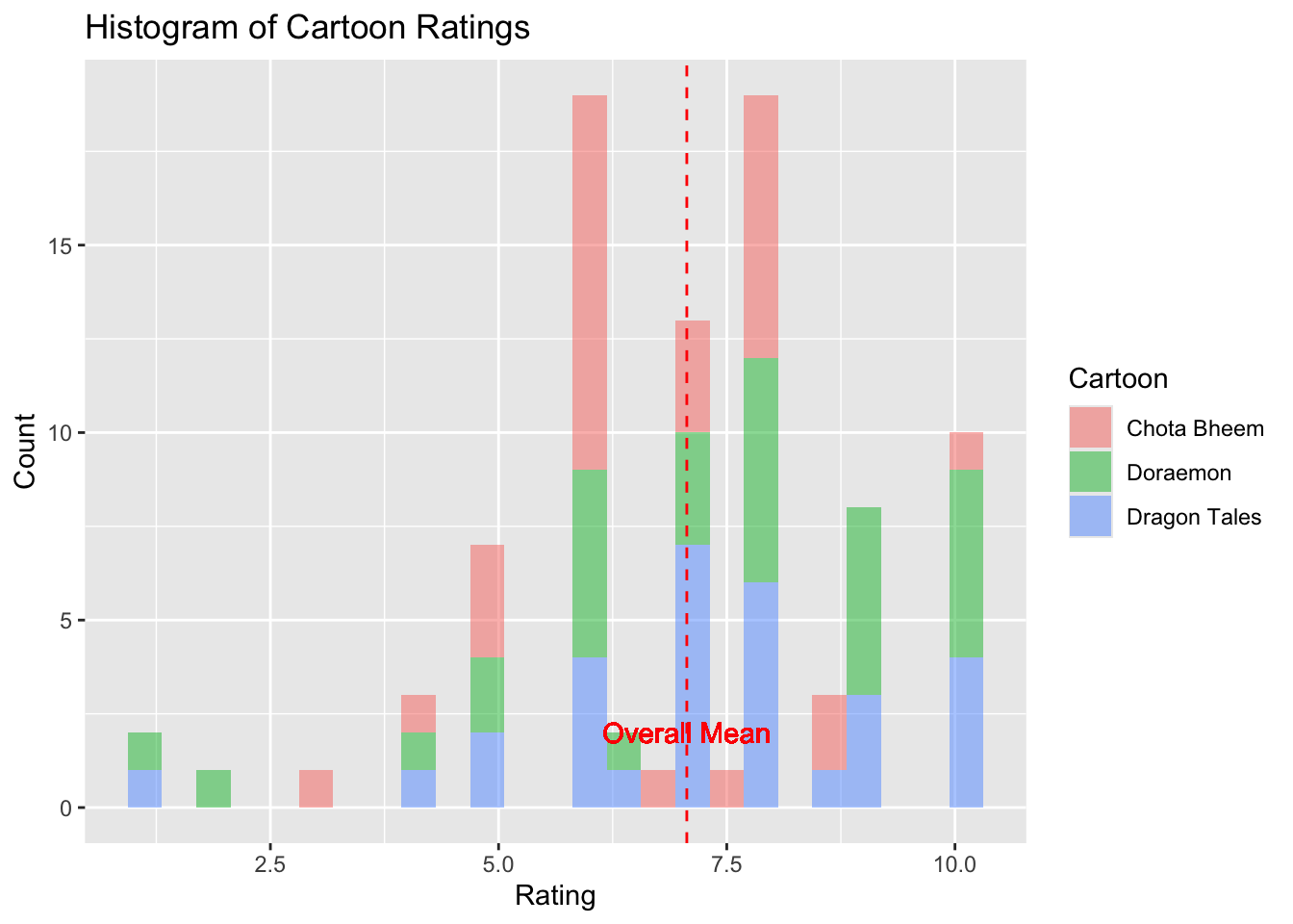
Plotting Graphs for Eda
gf_histogram(~Rating,
  fill = ~Cartoon,
  data = cartoons_modified,
  alpha = 0.5,
  bins = 25
) %>%
  gf_vline(xintercept = ~ mean(Rating, na.rm = TRUE),
            linetype = "dashed", color = "red") %>%
  gf_labs(
    title = "Histogram of Cartoon Ratings",
    x = "Rating",
    y = "Count"
  ) %>%
  gf_text(
    label = "Overall Mean",
    x = mean(cartoons_modified$Rating, na.rm = TRUE),
    y = 2,
    color = "red"
  ) %>%
  gf_refine(guides(fill = guide_legend(title = "Cartoon")))
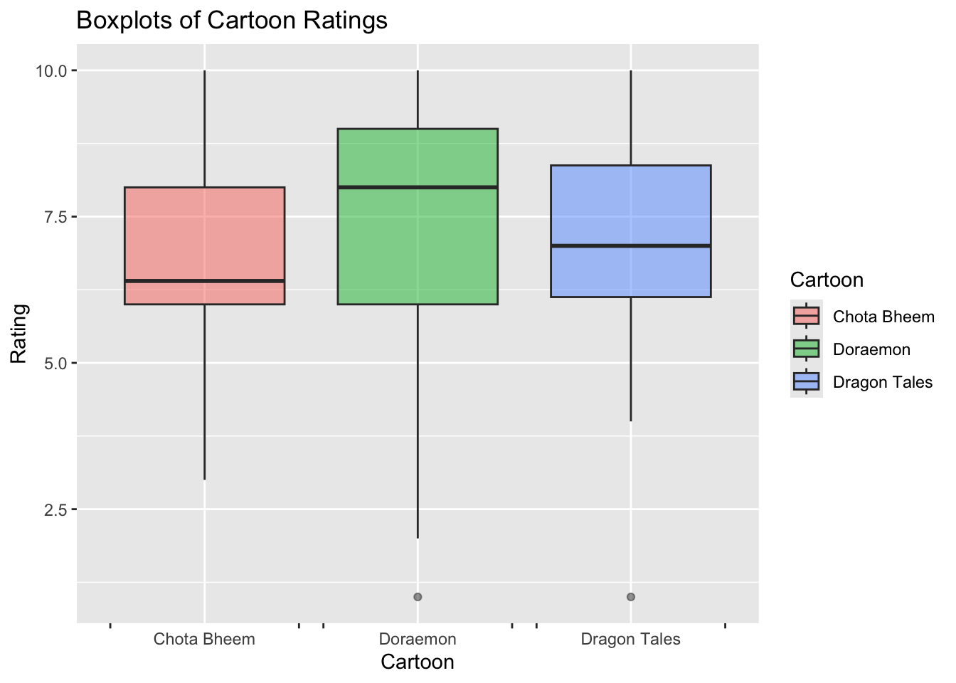
gf_boxplot(
  data = cartoons_modified,
  Rating ~ Cartoon,
  fill = ~Cartoon,
  alpha = 0.5
) %>%
  gf_vline(xintercept = ~ mean(Rating, na.rm = TRUE)) %>%
  gf_labs(
    title = "Boxplots of Cartoon Ratings",
    x = "Cartoon",
    y = "Rating",

  ) %>%
  gf_refine(
    scale_x_discrete(guide = "prism_bracket"),
    guides(fill = guide_legend(title = "Cartoon"))
  )
Warning: The S3 guide system was deprecated in ggplot2 3.5.0.
ℹ It has been replaced by a ggproto system that can be extended.
Observations
Doraemon with the highest mean seems to be the most popular, also shows wide variability
Dragon tales - less popular than the other two
Chota Bheem shows a smaller range of ratings
Outliers for Doraemon and Dragon tales
.
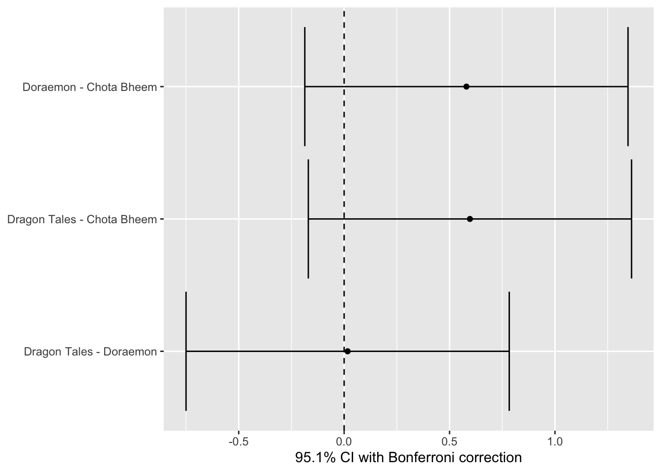
Anova
cartoon_anova <- aov(Rating ~ Cartoon, data = cartoons_modified)

supernova::pairwise(cartoon_anova,
  correction = "Bonferroni", # Try "Tukey"
  alpha = 0.05, # 95% CI calculation
  var_equal = TRUE, # We'll see
  plot = TRUE
)
── Pairwise t-tests with Bonferroni correction ─────────────────────────────────
Family-wise error-rate: 0.049
  group_1      group_2      diff pooled_se     t    df  lower upper  p_adj
  <chr>        <chr>       <dbl>     <dbl> <dbl> <int>  <dbl> <dbl>  <dbl>
1 Doraemon     Chota Bheem 0.580     0.354 1.636    87 -0.186 1.346  .3161
2 Dragon Tales Chota Bheem 0.597     0.354 1.683    87 -0.170 1.363  .2877
3 Dragon Tales Doraemon    0.017     0.354 0.047    87 -0.750 0.783 1.0000
Doraemon and Chota bheem have significantly different mean ratings.
Dragon Tales and Chota bheem have significantly different mean ratings.
There is no significant difference in mean ratings between Dragon Tales and Doraemon.
Doraemon is the highest rated followed by cHOTA bheem and then Dragon tales
supernova::equation(cartoon_anova)
Fitted equation:
Rating = 6.67 + 0.58*CartoonDoraemon + 0.5966667*CartoonDragon Tales + e
Checking Assumptions
Check for normality
shapiro.test(x = cartoons_modified$Rating)
    Shapiro-Wilk normality test

data:  cartoons_modified$Rating
W = 0.93517, p-value = 0.0002269
checking normality for each cartoon
normality_results <- cartoons_modified %>%
  group_by(Cartoon) %>%
  summarise(shapiro_p_value = shapiro.test(Rating)$p.value)

print(normality_results)
# A tibble: 3 × 2
  Cartoon      shapiro_p_value
  <fct>                  <dbl>
1 Chota Bheem           0.185
2 Doraemon              0.0139
3 Dragon Tales          0.0240
- based on p values, only the data for chota bheem is normally distributed
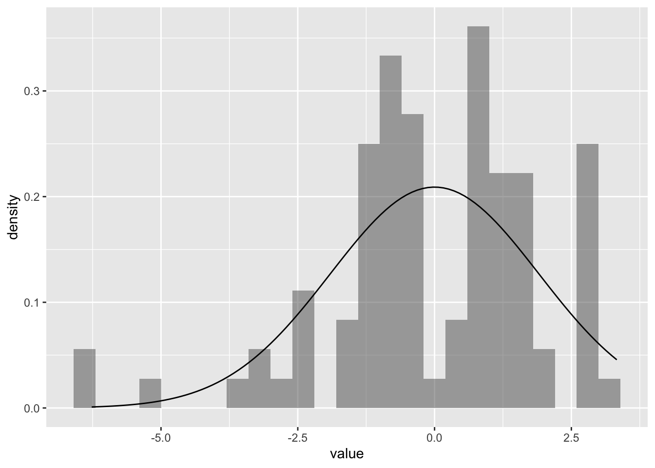
Residual post-model:
cartoon_anova$residuals %>%
  as_tibble() %>%
  gf_dhistogram(~value, data = .) %>%
  gf_fitdistr()
##
cartoon_anova$residuals %>%
  as_tibble() %>%
  gf_qq(~value, data = .) %>%
  gf_qqstep() %>%
  gf_qqline()
##
shapiro.test(cartoon_anova$residuals)
    Shapiro-Wilk normality test

data:  cartoon_anova$residuals
W = 0.93926, p-value = 0.0003856
- residuals are also not normally distributed
Check for Variance
cartoons_modified %>%
  group_by(Cartoon) %>%
  summarise(variance = var(Rating))
# A tibble: 3 × 2
  Cartoon      variance
  <fct>           <dbl>
1 Chota Bheem      2.21
2 Doraemon         5.25
3 Dragon Tales     3.84
# Perform Levene's Test for homogeneity of variances
DescTools::LeveneTest(Rating ~ Cartoon, data = cartoons_modified)
Levene's Test for Homogeneity of Variance (center = median)
      Df F value Pr(>F)
group  2  1.2923 0.2798
      87
# Perform Fligner-Killeen Test for homogeneity of variances
fligner.test(Rating ~ Cartoon, data = cartoons_modified)
    Fligner-Killeen test of homogeneity of variances

data:  Rating by Cartoon
Fligner-Killeen:med chi-squared = 1.8135, df = 2, p-value = 0.4038
both tests indicate that variances are approx equal.
Anova using permutation
observed_infer <-
  cartoons_modified %>%
  specify(Rating ~ Cartoon) %>%
  hypothesise(null = "independence") %>%
  calculate(stat = "F")

observed_infer
Response: Rating (numeric)
Explanatory: Cartoon (factor)
Null Hypothesis: independence
# A tibble: 1 × 1
   stat
  <dbl>
1 0.919
null_dist_infer <- cartoons_modified %>%
  specify(Rating ~ Cartoon) %>%
  hypothesise(null = "independence") %>%
  generate(reps = 4999, type = "permute") %>%
  calculate(stat = "F")
##
head(null_dist_infer, n = 15)
Response: Rating (numeric)
Explanatory: Cartoon (factor)
Null Hypothesis: independence
# A tibble: 15 × 2
   replicate   stat
       <int>  <dbl>
 1         1 0.530
 2         2 0.0222
 3         3 0.111
 4         4 0.108
 5         5 0.190
 6         6 0.310
 7         7 1.39
 8         8 1.27
 9         9 0.215
10        10 0.852
11        11 0.696
12        12 0.0170
13        13 0.566
14        14 0.792
15        15 2.90
##
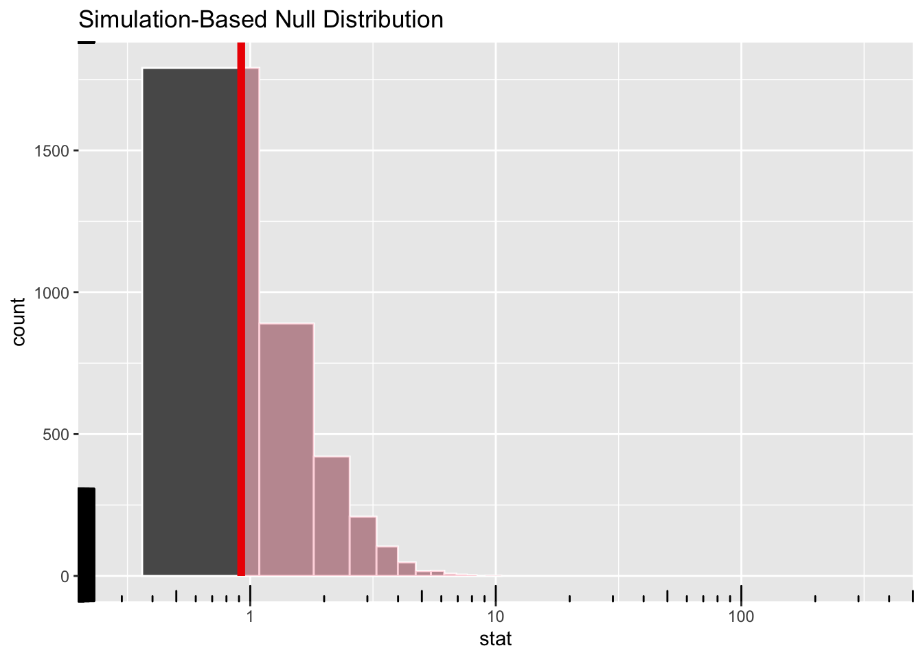
null_dist_infer %>%
visualise(method = "simulation") +
shade_p_value(obs_stat = observed_infer$stat, direction = "right") +
scale_x_continuous(trans = "log10", expand = c(0, 0)) +
coord_cartesian(xlim = c(0.2, 500), clip = "off") +
annotation_logticks(outside = FALSE)
Warning in transformation$transform(x): NaNs produced
Warning in scale_x_continuous(trans = "log10", expand = c(0, 0)): log-10
transformation introduced infinite values.
based on the infer based permutation test, the observed test statistic is not unusual and we fail to reject the null hypothesis- ???
Based on pairwise comparisons though…Doraemon > Chota Bheem > Dragon Tales